Pressures of Food Production

A team of experts in a working group at NCEAS put all food on the same table to assess and map the cumulative pressures of food prouction from ocean, aquatic, and terrestrial foods (crops and livestock).

The global assessment mapped the individual and cumulative pressures from climate emissions, nitrogen and phosphorous pollution, water use, and land/sea disturbance.

*Citation: Halpern, B.S., Frazier, M., Verstaen, J. et al. The environmental footprint of global food production. Nat Sustain 5, 1027–1039 (2022). https://doi.org/10.1038/s41893-022-00965-x

All data are available from KNB and the scripts are located on GitHub.

These global raster data describe the environmental footprint of the majority of food production for 2017.

We map four dominant global pressures of food production: disturbance (km2eq); blue freshwater consumption (m3 water); excess nutrients (tonnes NP); and greenhouse gas emissions (tonnes CO2eq). Categories of food include 26 crop categories (plus fodder, which is only consumed as feed); 6 livestock animals (cattle, buffalo, goats, sheep, pigs, chickens); 7 categories of marine fisheries, including forage fish species used for fishmeal and oil, other small pelagics, medium pelagics, large pelagics, benthic, demersal, and reef-associated; freshwater fisheries, with one group for all sizes and taxa; and 6 categories of marine aquaculture, including salmonids, unfed or algae fed shellfish, shrimp and prawns, tuna, other marine finfish, other crustaceans.

We primarily assess pressures from sources occurring within the farm-gate. In most cases, we exclude activities occurring beyond the farm-gate, such as processing and transportation of product, manufacture of equipment, and extraction of fuel because we were generally unable to map the location of these activities. For feed components, we map the pressures to the location where the crops are likely grown, after accounting for trade, or fish are captured (vs. where they are fed to animals).

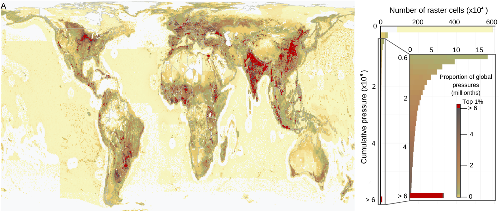
In addition to the raw data files, we also provide rescaled pressure data and a cumulative pressure index that combines the 4 pressures. To calculate the cumulative pressure, we adopted similar methods as other cumulative measures, rescaling each individual pressure (GHG, FW, NP, D) by dividing the values in each pixel (i) by the total global pressure summed across all food systems and pixels (T), such that each pixel describes its proportional contribution to the global total for that pressure. We then summed these rescaled pressure layers to obtain a total cumulative pressure score (CP) for each pixel i, such that CPi = GHGi/GHGT + FWi/FWT + NPi/NPT + Di/DT (raster cell values are multiplied by 1000000 to avoid small numbers and rounding errors). The result is that each rescaled pixel is a unitless value describing its proportional contribution to the total global pressure.

The cumulative pressure index allows direct comparisons among foods, regions, and pressures to identify where: individual pressures are high relative to other pressures, multiple pressures overlap, and hotspots of cumulative pressure are located. This information provides a more complete picture of the environmental pressures occurring at any global area and from each food type.

We us the Gall-Peters equal area coordinate reference system with a resolution of 36km2.

Other related projects

The theoretical background for mapping the environmental footprint of food is provided in Putting all foods on the same table: Achieving sustainable food systems requires full accounting and here.

We are now working to understand how the environmental pressures from food production might shift with changes to global diets, and to map how trade in food shifts footprints to distant locations and how that impacts diversity around the world.