Overview
CMIP6 Climate Scenario data: We are here to help!
Fri, Jan 28, 2022
If you are an ecologist or biologist and need data predicting future climate, then CMIP6 Scenario data may be what you are searching for! But, these data are big and complicated, and it can take some effort to understand them, especially if you are not a climate scientist.
In this blogpost, we describe these data so you can be on your way to responsibly using them (or, CMIP6 derived data) in your research to better predict how climate change will impact biological systems.
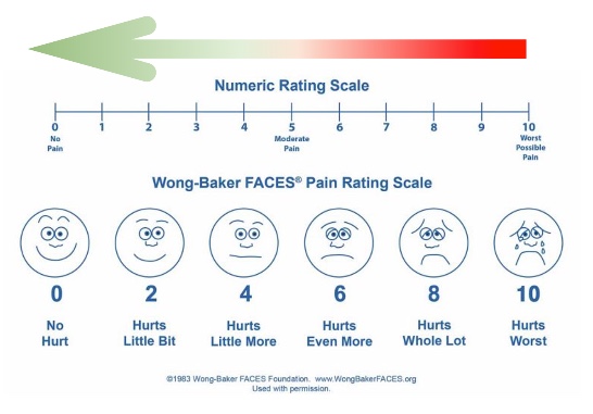
OUR GOAL: Reduce the pain of using CMIP6, or CMIP6-derived, data
This is the first blogpost of an upcoming series that will:
- Describe the CMIP6 Climate Scenario data (this post)
- Provide tips on obtaining and viewing raw data (future post) and finding ensemble data
- Describe approaches for working with raw CMIP6 data (future post)
Much of the content in this post is derived from these excellent sources:
-
ECMWF: A super useful and down-to-earth description of CMIP6!
-
Tebaldi, C., et al., 2021. Climate model projections from the Scenario Model Intercomparison Project (ScenarioMIP) of CMIP6. Earth System Dynamics 12, 253–293. https://doi.org/10.5194/esd-12-253-2021
What is CMIP6 Scenario data?
CMIP Phase 6 (i.e., Coupled Model Intercomparison Project) is a huge experiment coordinated by the World Climate Research Progam (WCRP) to predict the future of our climate. CMIP6 (as of 2022) is the most recent version of climate models and the outputs are used in the IPCC’s (Intergovernmental Panel on Climate Change) sixth assessment report.
CMIP6 is comprised of 23 CMIP6-Endorsed MIPs, but we focus only on the ScenarioMIP part of the project.
The ScenarioMIP project provides historical (1850-2014) climate projections and future climate projections (2015-2100) for eight different scenarios of emissions and land use change (see section: “CMIP6 Scenarios”).
Using this framework, independent institutions around the world (53 of them, in fact) model future climate using general circulation models which represent physical processes in the atmosphere, ocean, cryosphere, and land surface (ECMWF 2022). For example, near-surface air temperature models require information on radiation, convection, clouds, land characteristics, surface fluxes, as well as atmospheric circulation and turbulent transport. The centers use similar protocols with (mostly) the same input parameters (also known as “forcings”) and the best supported estimates of the sensitivity of climate to these forcings.
Because so many institutions are running simulations, many independent models are generated for each scenario and climate variable. By combining these independent, but standardized, outputs into ensembles we can, ideally, obtain better estimates of future climate change and get a better idea of the uncertainty in the estimates (See section: “Why Ensembles?”).
Forcing You will often see the word “Forcing” in climate literature. This refers to the variables that drive climate by affecting the flow of energy coming into and leaving the earth’s climate system. This includes variables such as solar radiation, green house gases, ozone, land use, volcanic eruptions.
Climate variables
Many different climate variables (e.g., sea surface temperature, near surface air temperature, rainfall) are modeled for the CMIP6 project. These data are available at various spatial and temporal levels:
- Different realms, including: land, atmosphere, and ocean.
- 2-d surface and 3-d data for a range of atmospheric air pressures and ocean depths.
- Various time intervals, including: monthly, daily, 3-hour intervals.
The climate variables often go by a short identifier. For example, to search for sea surface temperature data, you will often need to use it’s shortname which is “tos”. You can learn more about some of the common CMIP6 climate variables and their shortname (i.e., ESGF Variable ID) in the below table.
Click the triangle to see a long list of CMIP6 climate variables
Some common CMIP6 climate variables (from this incredibly helpful resource):
| Parameter name | �ESGF variable id | CDS parameter name for CMIP5 | Units |
|---|---|---|---|
| Near-surface air temperature | tas | 2m temperature | Kelvin |
| Daily maximum near-surface air temperature | tasmax | Maximum 2m temperature in the last 24 hours | Kelvin |
| Daily minimum near-surface air temperature | tasmin | Maximum 2m temperature in the last 24 hours | Kelvin |
| Surface temperature | ts | Skin temperature | Kelvin |
| Sea level pressure | psl | Mean sea level pressure | Pa |
| Surface air pressure | ps | Surface pressure | Pa |
| Eastward near-surface wind | uas | 10m u component of wind | m s-1 |
| Northward near-surface wind | vas | 10m v component of wind | m s-1 |
| Near-surface wind speed | sfcWind | 10m wind speed | m s-1 |
| Near-surface relative humidity | hurs | 2m relative humidity | 1 |
| Near-surface specific humidity | huss | 2m specific humidity | 1 |
| Precipitation | pr | Mean precipitation flux | kg m-2 s-1 |
| Snowfall flux | prsn | Snowfall | kg m-2 s-1 |
| Evaporation Including sublimation and transpiration | evspsbl | Evaporation | kg m-2 s-1 |
| Surface downward eastward wind stress | tauu | Eastward turbulent surface stress | Pa |
| Surface downward northward wind stress | tauv | Northward turbulent surface stress | Pa |
| Surface upward latent heat flux | hfls | Surface latent heat flux | W m-2 |
| Surface upward sensible heat flux | hfss | Surface sensible heat flux | W m-2 |
| Surface downwelling longwave radiation | rlds | Surface thermal radiation downwards | W m-2 |
| Surface upwelling longwave radiation | rlus | Surface upwelling longwave radiation | W m-2 |
| Surface downwelling shortwave radiation | rsds | Surface solar radiation downwards | W m-2 |
| Surface upwelling shortwave radiation | rsus | Surface upwelling shortwave radiation | W m-2 |
| TOA incident shortwave radiation | rsdt | TOA incident solar radiation | W m-2 |
| TOA outgoing shortwave radiation | rsut | TOA outgoing shortwave radiation | W m-2 |
| TOA outgoing longwave radiation | rlut | TOA outgoing longwave radiation | W m-2 |
| Total cloud cover percentage | clt | Total cloud cover | % |
| Air temperature | ta | Air temperature | K |
| Eastward wind | ua | U-component of wind | m s-1 |
| Northward wind | va | V-component of wind | m s-1 |
| Relative humidity | hur | Relative humidity | 1 |
| Specific humidity | hus | Specific humidity | 1 |
| Geopotential height | zg | Geopotential height | m |
| Surface snow amount | snw | Surface snow amount | kg m-2 |
| Snow depth | snd | Snow depth | m |
| Total runoff | mrro | Runoff | kg m-2 s-1 |
| Moisture in upper portion of soil column | mrsos | Soil moisture content | kg m-2 |
| Sea-Ice area percentage (ocean grid) | siconc | Sea-ice area percentage | 1 |
| Sea Ice thickness | sithick | Sea ice thickness | m |
| Sea-Ice mass per area | simass | Sea ice plus snow amount | kg m-2 |
| Surface temperature of sea Ice | sitemptop | Sea ice surface temperature | K |
| Sea surface temperature | tos | Sea surface temperature | K |
| Sea surface salinity | sos | Sea surface salinity | PSU |
| Sea surface height above geoid | zos | Sea surface height above geoid | m |
| Grid-cell area for ocean variables* | areacello | NOT AVAILABLE | m2 |
| Sea floor depth below geoid* | deptho | NOT AVAILABLE | m |
| Sea area percentage* | sftof | NOT AVAILABLE | % |
| Grid-cell area for atmospheric grid variables* | areacella | NOT AVAILABLE | m2 |
| Capacity of soil to store water (field capacity)* | mrsofc | NOT AVAILABLE | kg m-2 |
| Percentage of the grid cell occupied by land (including lakes)* | sftlf | NOT AVAILABLE | % |
| Land ice area percentage* | sftgif | NOT AVAILABLE | 1 |
| Surface altitude* | orog | NOT AVAILABLE | m |
You can also download a complete list of the CMIP6 climate data (data modified from this source). It is helpful to know that the climate variables are organized into separate tables, for example monthly ocean data can mostly be found in Omon table. A list of the tables is provided on the first tab. There are LOTS of tables, and the organization isn’t immediately intuitive (at least to me).
All Climate variablesCMIP6 Scenarios
Predicting future climate requires making underlying predictions about how our world might look in the future.
The IPCC Sixth Assessment Report (CMIP6) includes 8 future scenarios (2015-2100) and one historical scenario (1850-2014). The CMIP6 scenarios combine two frameworks: the Shared Socioeconomic Pathway (SSP, first part of the scenario name) and the Representative Concentration Pathway (RCP, second part of the scenario name).
Shared Socioeconomic Pathways (SSPs) describe 5 potential pathways of global socioeconomic development, based on variables such as population, technological advancements, climate policies, and gross domestic product. These storylines are then used to determine the likely consequences of these developments on anthropogenic emissions and land-use. This paper describes the concept behind SSPs.
RCPs describe specific radiative forcing endpoints by 2100 based on future concentrations of emissions. RCPs were first used in the Fifth IPCC assessment. For continuity, the current CMIP6 scenarios includes the original 4 RCP categories from the Fifth Assessment, but the current framework aligns these with SSP categories and fills in some RCP gaps (e.g., SSP-RCP). Note that an SSP scenario may have multiple potential RCPs.
These pathways are defined by the concentration of carbon in the atmosphere and not the volume of emissions. Models based on concentration scenarios do not include climate feedbacks that are likely to exacerbate warming, such as: the release of methane if permafrost melts, disruptions to ocean circulation, rainforest drought and loss, etc. Warming predictions tend to be higher under emission-based scenarios that take into account some carbon cycle feedbacks.
Scenarios included in CMIP6
This information is from here and here.
| IPCC Scenarios | Description | Estimated Warming 2041-2060, C |
|---|---|---|
| historical | Simulation of climate variables from the recent past from 1850 to 2014. These predictions are from a coupled atmosphere-ocean general circulation model (AOGCM) using observed variables such as atmospheric composition, land use and solar forcing. The historical simulation can be used to evaluate model performance against present climate and observed climate change. | NA |
| SSP1-1.9 | Based on SSP1 with low climate change mitigation and adaptation challenges which leads to a future pathway with a radiative forcing of 1.9 W/m2 in the year 2100. The SSP1-1.9 scenario fills a gap at the very low end of the range of plausible future forcing pathways, due to interest in informing a possible goal of limiting global mean warming to 1.5°C above pre-industrial levels based on the Paris COP21 agreement. | 1.6 |
| SSP1-2.6 | Based on SSP1 with low climate change mitigation and adaptation challenges which leads to a radiative forcing of 2.6 W/m2 in the year 2100. The SSP1-2.6 scenario represents the low end of plausible future forcing pathways. SSP1-2.6 depicts a “best case” future from a sustainability perspective. | 1.7 |
| SSP4-3.4 | Based on SSP4 in which climate change adaptation challenges dominate which leads to a radiative forcing of 3.4 W/m2 in the year 2100. The SSP4-3.4 scenario fills a gap at the low end of the range of plausible future forcing pathways. SSP4-3.4 is of interest to mitigation policy since mitigation costs differ substantially between forcing levels of 4.5 W/m2 and 2.6 W/m2. | |
| SSP5-3.4OS | Based on SSP5 in which climate change mitigation challenges dominate with a peak and decline in forcing towards an eventual radiative forcing of 3.4 W/m2 in the year 2100. The SSP5-3.4OS scenario branches from SSP5-8.5 in the year 2040 whereupon it applies substantially negative net emissions. SSP5-3.4OS explores the climate science and policy implications of a peak and decline in forcing during the 21st century. SSP5-3.4OS fills a gap in existing climate simulations by investigating the implications of a substantial overshoot in radiative forcing relative to a longer-term target. | |
| SSP2-4.5 | Based on SSP2 with intermediate climate change mitigation and adaptation challenges which lead to a radiative forcing of 4.5 W/m2 in the year 2100. The SSP2-4.5 scenario represents the medium part of plausible future forcing pathways. SSP2-4.5 is comparable to the CMIP5 experiment RCP4.5. | 2.0 |
| SSP4-6.0 | SSP4-6.0 is based on SSP4 in which climate change adaptation challenges dominate and RCP6.0 which lead to a radiative forcing of 6.0 W/m2 in the year 2100. The SSP4-6.0 scenario fills in the range of medium plausible future forcing pathways. SSP4-6.0 defines the low end of the forcing range for unmitigated SSP baseline scenarios. | |
| SSP3-7.0 | Based on SSP3 in which climate change mitigation and adaptation challenges are high which leads to a radiative forcing of 7.0 W/m2 in the year 2100. The SSP3-7.0 scenario represents the medium to high end of plausible future forcing pathways. SSP3-7.0 fills a gap in the CMIP5 forcing pathways that is particularly important because it represents a forcing level common to several (unmitigated) SSP baseline pathways. | 2.1 |
| SSP5-8.5 | SSP5-8.5 is based on SSP5 in which climate change mitigation challenges dominate which leads to a radiative forcing of 8.5 W/m2 in the year 2100. The ssp585 scenario represents the high end of plausible future forcing pathways. SSP5-8.5 is comparable to the CMIP5 experiment RCP8.5. | 2.4 |
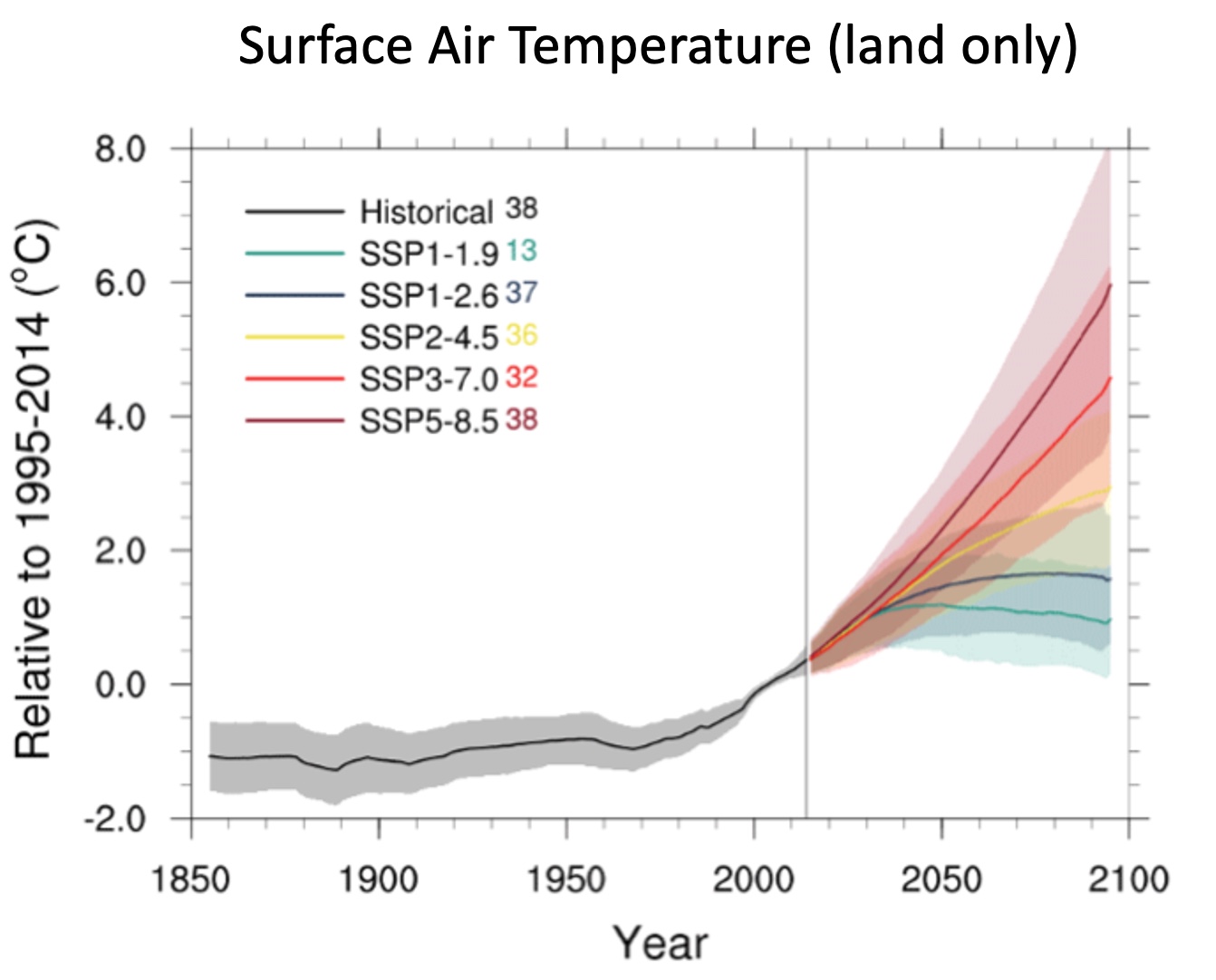
This plot shows how future surface air temperature is predicted to increase for 5 CMIP6 scenarios (from: https://esd.copernicus.org/articles/12/253/2021/). The numbers included in the legend describe the number of models included in each scenario. The dark line indicates the mean of the models. Note that the historical predictions are also included.
Click the triangle to learn more about Shared Socioeconomic Pathways and Representative Concentration Pathways
Shared Socioeconomic Pathways
Under the Shared Socioeconomic Pathway (SSP) framework, human society may develop along several pathways that have different implications for future climate change. SSP considers potential changes in social progress, inequality, global markets, innovation, and consumption of fossil fuels, and other variables.
Shared Socioeconomic Pathway Narratives from Wikipedia.
[WARNING: Most of these pathways are feasible AND depressing].
| Shared Socioeconomic Pathway | Description |
|---|---|
| SSP1: Sustainability (…this one..please!) | The world slowly shifts to a more sustainable path. Increased investment in education and health, and a transition from economic growth to human well-being. Inequality is reduced within and across countries. |
| SSP2: Middle of the road | The world mostly continues down its current trajectory with little change in social, economic, and technological trends. Improvements to human well-being, environmental systems, resource use, and sustainability progress unevenly within and across countries. |
| SSP3: Regional rivalry | Regional rivalries, nationalistic tendancies, and concerns about national security result in countries investing heavily in military and food security. This comes at the expense of addressing large scale global environmental concerns and investing in education and technological development. |
| SSP4: Inequality | Highly unequal investments in human capital, combined with increasing disparities in economic opportunity and political power, lead to increasing inequalities and stratification both across and within countries. The depressing result is that social cohesion breaks down and conflict and unrest become increasingly common. Environmental issues are not addressed at the global scale, but instead address local issues in richer areas. |
| SSP5: Fossil-Fueled Development | Rapid economic and social development that is sustained by resource and energy intensive lifestyles around the world. The global economy grows along with green house gas emissions. Local environmental problems are managed, but greenhouse gas emissions are essentially uncontrolled. |
Representative Concentration Pathways
Representative Concentration Pathways describe likely future climate scenarios in units of radiative forcing, W/m2, in the year 2100 (https://en.wikipedia.org/wiki/Radiative_forcing). For the IPCC’s Fifth Assessement Report (2014), 4 Representative Concentration Pathways (RCP 2.6, 4.5, 6, 8.5) were chosen to represent the range of possible possible climate outcomes due to future anthropogenic greenhouse gas emissions.
What scenarios should I use???!
All of them! [At least in the ideal world.]
In the real world, there are limits on time and computational resources. And, depending on your project goals, there is likely to be diminishing returns by running all scenarios. This is a complicated question, and it depends on what you are trying to accomplish, but a recent paper (Burgess et al. 2022) provides a useful perspective for thinking about this issue:
Download paperAlthough emissions pathways are subject to deep uncertainty, recent research suggests that emissions scenarios producing a range of approximately 3.4-4.5W/m2 radiative forcing by 2100 might be most plausible. With median climate sensitivities, this corresponds to approximately 2-3 degrees C global warming by 2100. Climate-sensitivity uncertainties expand this range to approximately 1.5-4 degrees C. In terms of the Shared Socioeconomic Pathways (SSPs) and Representative Concentration Pathways (RCPs), radiative forcing outcomes mostly fall between SSP2-3.4 and SSP2-4.5/RCP4.5, though higher and lower emissions scenarios (e.g., RCP2.6 and RCP6.0) might be plausible and should be explored in research. However, we argue that uses of the highest-emission scenarios (RCP8.5/SSP5-8.5, SSP3-7.0)—which currently predominate the literature—should come with clearly articulated rationales and appropriate caveats to ensure results are not misinterpreted by scholars, policymakers, and media.
And, this post discusses whether RCP8.5 is a good prediction of future warming, or, is a worst case scenario. Spoiler Alert: This depends on what green house gas emissions look like in the future and how carbon/warming feedback loops play out (which is particularly difficult to predict).
Historical vs. Future Data
Along with future predictions, the CMIP6 scenario data provides modeled historical data. The historical scenario data are generated using the same General Circulation Models used to generate the future scenarios. There is a fair amount of variation around the predicted historical data among the different climate models (see the scenario figure above, specifically the gray shaded area of historical region), especially as you go back further in time. These data are handy for determining how well particular models are working.
The best way to use the CMIP historical data can be confusing! When it comes to using the historical data, it feels like datasets based on observed measurements should be preferable to fully modeled data (like that from CMIP). AND: This is true if you are comparing near-historical climate data to current climate data!! BUT, if you want to compare current climate to future climate then you should use CMIP historical data for these comparisons.
In short: If you are comparing current climate to future climate, you should use the corresponding CMIP historical data for these comparisons!
If you want to understand current climate pressures relative to the past, then CMIP historical data probably isn’t your best choice! Instead, a good option may be the ERA5 data, which combines observational and model data!
Why Ensembles?
A SERVICE ANNOUNCEMENT: If you are a researcher creating ensemble models PLEASE PLEASE make the output data available! Providing a PNG of the results does not count. And, neither does citing the ESFG website that provides the raw climate data. Thanks from all of us! :)
The CMIP6 process generates many models for each scenario and climate variable. The mean of all, or a subset, of these models generally provides a better climate estimate than any given individual model (e.g., below figure, solid lines for each scenario). And, the range spanned by the models can be interpreted as an estimate of scenario uncertainty (e.g., below figure, shaded portions around means).
In addition to all the climate centers producing independent models, a single climate center can have multiple “ensemble members” (these have names like: r1i1p1f1) that vary in regard to initial model starting conditions. Some models only have one member. Five models (CanESM5, IPSL-CM6A-LR, MPI-ESM1-2-HR, MPI-ESM1-2-LR and UKESM1) have at least 10 ensemble members for some scenarios. The CanESM5 has an impressive 50 ensemble members. This is kind of cool because provides two levels of variation that can be explored!
The overall idea of an ensemble is simple, but there are two critical things to keep in mind:
-
Models should only be averaged within a scenario (e.g., do not combine models from different scenarios)
-
To the extent possible, each scenario that an ensemble is calculated for should include the same climate models
Beyond this general advice, there are many additional things to consider:
-
What is the best way to deal with the “ensemble members” generated by a single climate center/model? In some cases, these within-model ensemble members are averaged. In other cases, a representative ensemble member is selected (often r1i1p1f1 because it’s the most commonly available across models).
-
What models should be included? This seems to vary from about 5 to all of them! There are a lot of thoughts, for [example] (https://www.jstage.jst.go.jp/article/sola/17/0/17_2021-009/_article) on this.
-
Should the contributions of the models be weighted? Historically, the models have been equally weighted, but models have weighted the models based on their independence from other models as well as how well they predict historical conditions.
Where do I get the data?
If you are an ecologist or biologist who wants climate predictions to understand impacts on organisms or ecological systems (vs. someone who is actually studying climate) ideally you will be able to download premade ensembles, and not have to deal with raw climate data! We hope that you will be able to minimize your contact with the raw data (unlesss you love this kind of thing). But if you have to resort to the raw data, the next posts will be helpful.
Even if you do not use raw CMIP6 data, I recommend taking a quick look at the websites that distribute the data because this can be helpful for understanding the data. And, if you need more information, we will guide you through the process of obtaining raw CMIP6 data in the next post.
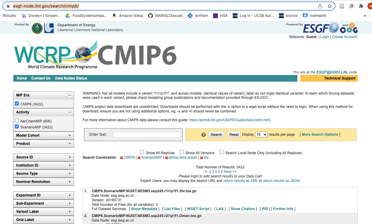
The CMIP6 data archive is distributed through the Earth System Grid Federation (ESGF)
The Climate Data Store (CDS) also provides a quality-controlled subset of the wider CMIP6 data. This quality control procedure ensures a high standard of dependability of the data, in contrast to the ESGF archive which comes “with very limited quality assurance and may have metadata errors or omissions."(from: https://confluence.ecmwf.int/display/CKB/CMIP6%3A+Global+climate+projections)
The Climate Data Store has a user interface that is much easier to use that the ESGF website and there is an API for programmatically downloading the data that I was able to use fairly quickly. However, it is possible to encounter long queue times to get the data.
The Climate Data Store also provides climate extreme data derived from CMIP6.
References
-
https://confluence.ecmwf.int/display/CKB/CMIP6%3A+Global+climate+projections
-
ECMWF: A super useful and down-to-earth description of CMIP6!
-
Tebaldi, C., et al., 2021. Climate model projections from the Scenario Model Intercomparison Project (ScenarioMIP) of CMIP6. Earth System Dynamics 12, 253–293. https://doi.org/10.5194/esd-12-253-2021
This post was created as part of the MARISCO project which is funded by the Belmont Forum.
Belmont Forum members and partner organizations work together to direct and fund research on environmental change that affect us all.