Overview
CMIP6 Climate Scenario data: Where do I get the data!
Fri, Dec 16, 2022
If you are an ecologist or biologist and need predictions of future climate variables, then the CMIP6 Scenario data will probably be what you want!
In this blogpost, we provide an overview of the raw CMIP6 data because this is helpful for understanding these data. However, because we believe non-climate scientists should probably seek more derived CMIP6 products, we also provide information about some of these products that we have used in our research.
A previous post provides an overview of the CMIP6 Scenario data. If you are new to CMIP data, we recommend starting there. This article, “CMIP6: the next generation of climate models explained” also provides an excellent overview of CMIP6 that manages to be high-level and understandable. And, much of the content in this post is derived from this excellent source, which I highly recommend reading because it provides a super useful and down-to-earth description of CMIP6.
We are always on the hunt for data. Please let us know (frazier@nceas.ucsb.edu) if you discover CMIP6 ensemble datasets and/or downscaled data that are publicly available. I will add them to this post. MANY THANKS!
Raw CMIP data
Earth System Grid Federation: A deep dive
The CMIP6 data archive is distributed through the Earth System Grid Federation (ESGF).
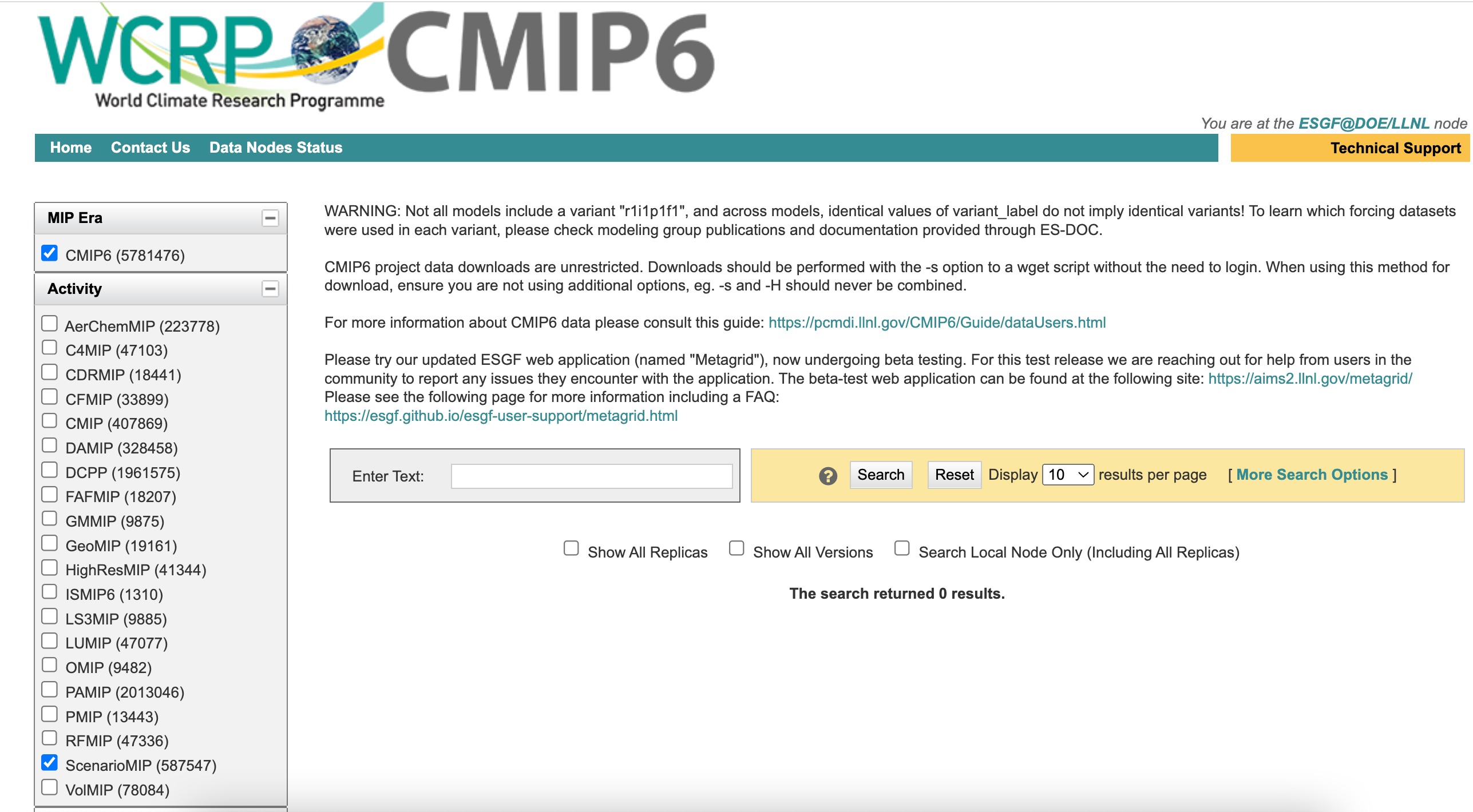
If the ESGF website seems daunting, don’t worry, we feel the same!
There are a series of dropdown menus on the left of the ESGF site that will guide you through the process of finding data. We recommend an iterative approach because if the “Search” button is clicked after selecting a menu option, the subsequent menus will be simplified as irrelevant categories are removed.
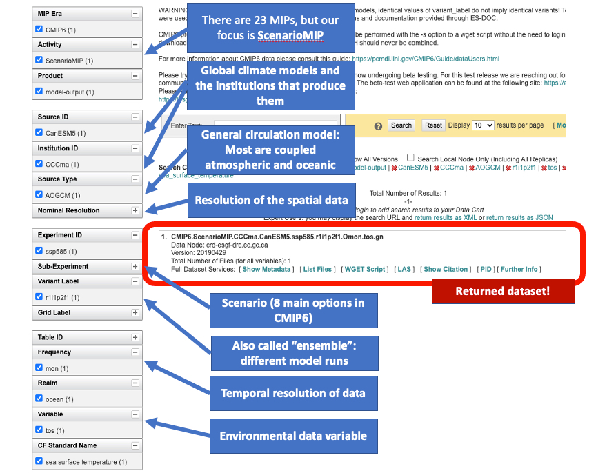
Source ID & Institution ID
The global climate models and institutions that produce them. I usually skip over this section because it is rare for me to select on the model, and depending on the climate variable of interest, many of these options will disappear.
Click the triangle to see all the climate models and institutions
CMIP6 data models and institutions (from this incredibly helpful resource):
| goal | 2012 | 2013 | 2014 | 2015 | 2016 | 2017 | 2018 | 2019 | 2020 | 2021 | 2022 | |
|---|---|---|---|---|---|---|---|---|---|---|---|---|
| 1 | Index | 69.4 | 69.9 | 70.3 | 70.6 | 70.7 | 70.4 | 70.4 | 70 | 68.8 | 69 | 69.2 |
| 2 | Artisanal opportunities | 75.8 | 76.3 | 76.7 | 76.7 | 75.9 | 75.1 | 75.1 | 74.9 | 75.4 | 74.8 | 77.1 |
| 3 | Species condition (subgoal) | 79.7 | 79.5 | 79.3 | 79.1 | 78.9 | 78.7 | 78.5 | 78.3 | 78.1 | 77.9 | 77.7 |
| 4 | Biodiversity | 79 | 78.5 | 78 | 78.2 | 77.9 | 77.4 | 77.1 | 76.7 | 76.4 | 76.3 | 76.3 |
| 5 | Habitat (subgoal) | 78.4 | 77.5 | 76.8 | 77.4 | 76.8 | 76.1 | 75.7 | 75.1 | 74.7 | 74.8 | 74.9 |
| 6 | Coastal protection | 82.6 | 82.5 | 82.6 | 82.6 | 82.7 | 82.2 | 81.9 | 81.7 | 81.8 | 81.9 | 82.3 |
| 7 | Carbon storage | 81 | 81 | 81 | 81 | 81 | 81 | 81 | 81.1 | 81.1 | 81 | 81 |
| 8 | Clean water | 67.7 | 67.6 | 68.5 | 68.8 | 69.2 | 69.3 | 69.4 | 69 | 69.2 | 70.2 | 70.2 |
| 9 | Fisheries (subgoal) | 53.7 | 54.4 | 54.9 | 54.8 | 54.1 | 53.8 | 53.4 | 53.5 | 53.5 | 53.4 | 53.4 |
| 10 | Food provision | 50.6 | 50.9 | 51.3 | 51.2 | 50.5 | 50.1 | 49.8 | 49.8 | 49.8 | 49.6 | 49.5 |
| 11 | Mariculture (subgoal) | 5.7 | 5.6 | 5.6 | 5.7 | 5.8 | 5.9 | 6 | 6.1 | 6.2 | 6.4 | 6.6 |
| 12 | Iconic species (subgoal) | 64 | 65 | 65 | 65.5 | 64.7 | 64.6 | 65.5 | 62.7 | 60.3 | 59.8 | 59.7 |
| 13 | Sense of place | 59.4 | 60 | 60.8 | 61.2 | 61.5 | 62.4 | 63.6 | 62.6 | 61.4 | 61.3 | 61 |
| 14 | Lasting special places (subgoal) | 54.8 | 55 | 56.6 | 57 | 58.2 | 60.1 | 61.6 | 62.6 | 62.5 | 62.7 | 62.3 |
| 15 | Natural products | 76.1 | 76 | 77.4 | 78.2 | 78.5 | 78.3 | 77 | 75.7 | 76 | 75.1 | 74.9 |
| 16 | Tourism & recreation | 44.5 | 45.6 | 46.3 | 47.4 | 49 | 48 | 48.4 | 48.1 | 35.3 | 38.5 | 38.8 |
Source Type
A description of the general circulation model. In most cases, the model is a coupled atmospheric and oceanic general circulation model (AOGCM), but other models are used.
Atmospheric (AGCMs) and oceanic GCMs (OGCMs) can be coupled to form an atmosphere-ocean coupled general circulation model (CGCM or AOGCM). With the addition of submodels such as a sea ice model or a model for evapotranspiration over land, AOGCMs become the basis for a full climate model. – Wikipedia
Experiment ID (aka “scenarios”)
The IPCC Sixth Assessment Report (CMIP6) includes 8 future scenarios (2015-2100) and one historical scenario (1850-2014). These scenarios represent different pathways the world might follow, which will lead to different predictions of future climate.
Click the triangle to see the climate scenarios
CMIP6 data climate scenarios (from this incredibly helpful resource) and here.
| IPCC Scenarios | Description | Estimated Warming 2041-2060, C |
|---|---|---|
| historical | Simulation of climate variables from the recent past from 1850 to 2014. These predictions are from a coupled atmosphere-ocean general circulation model (AOGCM) using observed variables such as atmospheric composition, land use and solar forcing. The historical simulation can be used to evaluate model performance against present climate and observed climate change. | NA |
| SSP1-1.9 | Based on SSP1 with low climate change mitigation and adaptation challenges which leads to a future pathway with a radiative forcing of 1.9 W/m2 in the year 2100. The SSP1-1.9 scenario fills a gap at the very low end of the range of plausible future forcing pathways, due to interest in informing a possible goal of limiting global mean warming to 1.5°C above pre-industrial levels based on the Paris COP21 agreement. | 1.6 |
| SSP1-2.6 | Based on SSP1 with low climate change mitigation and adaptation challenges which leads to a radiative forcing of 2.6 W/m2 in the year 2100. The SSP1-2.6 scenario represents the low end of plausible future forcing pathways. SSP1-2.6 depicts a “best case” future from a sustainability perspective. | 1.7 |
| SSP4-3.4 | Based on SSP4 in which climate change adaptation challenges dominate which leads to a radiative forcing of 3.4 W/m2 in the year 2100. The SSP4-3.4 scenario fills a gap at the low end of the range of plausible future forcing pathways. SSP4-3.4 is of interest to mitigation policy since mitigation costs differ substantially between forcing levels of 4.5 W/m2 and 2.6 W/m2. | |
| SSP5-3.4OS | Based on SSP5 in which climate change mitigation challenges dominate with a peak and decline in forcing towards an eventual radiative forcing of 3.4 W/m2 in the year 2100. The SSP5-3.4OS scenario branches from SSP5-8.5 in the year 2040 whereupon it applies substantially negative net emissions. SSP5-3.4OS explores the climate science and policy implications of a peak and decline in forcing during the 21st century. SSP5-3.4OS fills a gap in existing climate simulations by investigating the implications of a substantial overshoot in radiative forcing relative to a longer-term target. | |
| SSP2-4.5 | Based on SSP2 with intermediate climate change mitigation and adaptation challenges which lead to a radiative forcing of 4.5 W/m2 in the year 2100. The SSP2-4.5 scenario represents the medium part of plausible future forcing pathways. SSP2-4.5 is comparable to the CMIP5 experiment RCP4.5. | 2.0 |
| SSP4-6.0 | SSP4-6.0 is based on SSP4 in which climate change adaptation challenges dominate and RCP6.0 which lead to a radiative forcing of 6.0 W/m2 in the year 2100. The SSP4-6.0 scenario fills in the range of medium plausible future forcing pathways. SSP4-6.0 defines the low end of the forcing range for unmitigated SSP baseline scenarios. | |
| SSP3-7.0 | Based on SSP3 in which climate change mitigation and adaptation challenges are high which leads to a radiative forcing of 7.0 W/m2 in the year 2100. The SSP3-7.0 scenario represents the medium to high end of plausible future forcing pathways. SSP3-7.0 fills a gap in the CMIP5 forcing pathways that is particularly important because it represents a forcing level common to several (unmitigated) SSP baseline pathways. | 2.1 |
| SSP5-8.5 | SSP5-8.5 is based on SSP5 in which climate change mitigation challenges dominate which leads to a radiative forcing of 8.5 W/m2 in the year 2100. The ssp585 scenario represents the high end of plausible future forcing pathways. SSP5-8.5 is comparable to the CMIP5 experiment RCP8.5. | 2.4 |
Variant Label
Modeling centers often run the same climate model with slightly different settings and initial conditions. A model and its collection of runs is referred to as an ensemble (not to be confused with “ensembles” that combine the various climate models, typically from different institutions). For some models, there is only one variant, but some models (e.g., CanESM5) include large numbers of variants.
These are interesting from a statistical perspective because they give some idea of the variation at this modeling scale.
Click the triangle to learn more about these ensembles
CMIP6 esembles (taken entirely from this incredibly helpful resource): Within these ensembles, four different categories of sensitivity studies are done, and the resulting individual model runs are labelled by four integers indexing the experiments in each category
e.g. r
- The first category, labelled realization_index (referred to with letter r), performs experiments which differ only in random perturbations of the initial conditions of the experiment. Comparing different realizations allow estimation of the internal variability of the model climate.
- The second category, labelled initialization_index (referred to with letter i), refers to variation in initialisation parameters. Comparing differently initialised output provides an estimate of how sensitive the model is to initial conditions.
- The third category, labelled physics_index (referred to with letter p), refers to variations in the way in which sub-grid scale processes are represented. Comparing different simulations in this category provides an estimate of the structural uncertainty associated with choices in the model design.
- The fourth category labelled forcing_index (referred to with letter f) is used to distinguish runs of a single CMIP6 experiment, but with different forcings applied.
Variable
Many different climate variables (e.g., sea surface temperature, near surface air temperature, rainfall) are modeled for the CMIP6 project.
The climate variables often go by a short identifier. For example, to search for sea surface temperature data, you will often need to use it’s shortname which is “tos”. You can learn more about some of the common CMIP6 climate variables and their shortname (i.e., ESGF Variable ID) in the below table.
Click the triangle to see a long list of CMIP6 climate variables
Some common CMIP6 climate variables (from this incredibly helpful resource):
| Parameter name | �ESGF variable id | CDS parameter name for CMIP5 | Units |
|---|---|---|---|
| Near-surface air temperature | tas | 2m temperature | Kelvin |
| Daily maximum near-surface air temperature | tasmax | Maximum 2m temperature in the last 24 hours | Kelvin |
| Daily minimum near-surface air temperature | tasmin | Maximum 2m temperature in the last 24 hours | Kelvin |
| Surface temperature | ts | Skin temperature | Kelvin |
| Sea level pressure | psl | Mean sea level pressure | Pa |
| Surface air pressure | ps | Surface pressure | Pa |
| Eastward near-surface wind | uas | 10m u component of wind | m s-1 |
| Northward near-surface wind | vas | 10m v component of wind | m s-1 |
| Near-surface wind speed | sfcWind | 10m wind speed | m s-1 |
| Near-surface relative humidity | hurs | 2m relative humidity | 1 |
| Near-surface specific humidity | huss | 2m specific humidity | 1 |
| Precipitation | pr | Mean precipitation flux | kg m-2 s-1 |
| Snowfall flux | prsn | Snowfall | kg m-2 s-1 |
| Evaporation Including sublimation and transpiration | evspsbl | Evaporation | kg m-2 s-1 |
| Surface downward eastward wind stress | tauu | Eastward turbulent surface stress | Pa |
| Surface downward northward wind stress | tauv | Northward turbulent surface stress | Pa |
| Surface upward latent heat flux | hfls | Surface latent heat flux | W m-2 |
| Surface upward sensible heat flux | hfss | Surface sensible heat flux | W m-2 |
| Surface downwelling longwave radiation | rlds | Surface thermal radiation downwards | W m-2 |
| Surface upwelling longwave radiation | rlus | Surface upwelling longwave radiation | W m-2 |
| Surface downwelling shortwave radiation | rsds | Surface solar radiation downwards | W m-2 |
| Surface upwelling shortwave radiation | rsus | Surface upwelling shortwave radiation | W m-2 |
| TOA incident shortwave radiation | rsdt | TOA incident solar radiation | W m-2 |
| TOA outgoing shortwave radiation | rsut | TOA outgoing shortwave radiation | W m-2 |
| TOA outgoing longwave radiation | rlut | TOA outgoing longwave radiation | W m-2 |
| Total cloud cover percentage | clt | Total cloud cover | % |
| Air temperature | ta | Air temperature | K |
| Eastward wind | ua | U-component of wind | m s-1 |
| Northward wind | va | V-component of wind | m s-1 |
| Relative humidity | hur | Relative humidity | 1 |
| Specific humidity | hus | Specific humidity | 1 |
| Geopotential height | zg | Geopotential height | m |
| Surface snow amount | snw | Surface snow amount | kg m-2 |
| Snow depth | snd | Snow depth | m |
| Total runoff | mrro | Runoff | kg m-2 s-1 |
| Moisture in upper portion of soil column | mrsos | Soil moisture content | kg m-2 |
| Sea-Ice area percentage (ocean grid) | siconc | Sea-ice area percentage | 1 |
| Sea Ice thickness | sithick | Sea ice thickness | m |
| Sea-Ice mass per area | simass | Sea ice plus snow amount | kg m-2 |
| Surface temperature of sea Ice | sitemptop | Sea ice surface temperature | K |
| Sea surface temperature | tos | Sea surface temperature | K |
| Sea surface salinity | sos | Sea surface salinity | PSU |
| Sea surface height above geoid | zos | Sea surface height above geoid | m |
| Grid-cell area for ocean variables* | areacello | NOT AVAILABLE | m2 |
| Sea floor depth below geoid* | deptho | NOT AVAILABLE | m |
| Sea area percentage* | sftof | NOT AVAILABLE | % |
| Grid-cell area for atmospheric grid variables* | areacella | NOT AVAILABLE | m2 |
| Capacity of soil to store water (field capacity)* | mrsofc | NOT AVAILABLE | kg m-2 |
| Percentage of the grid cell occupied by land (including lakes)* | sftlf | NOT AVAILABLE | % |
| Land ice area percentage* | sftgif | NOT AVAILABLE | 1 |
| Surface altitude* | orog | NOT AVAILABLE | m |
Resources for derived products
We’ve said this before, but we’ll say it again: If you are an ecologist or biologist you should, if possible, avoid the raw climate data and use more derived products that others have created.
Using derived products can provide many advantages:
Derived data products are generally easier to work with because the raw ESGF has many idiosyncrasy’s. One example: data are often reported using an irregular grid that must be interpolated to a regular grid.
You will be able to harness the power of the ensemble! Most derived CMIP6 data products are “ensembles” that combine a subset of the CMIP6 climate models into a single dataset. In most cases, ensembles are more accurate than any given single climate model.
Much of the raw CMIP data is very coarse resolution (e.g., 1 to 1.25 degrees). You may be able to find downscaled climate data which has translated coarse resolution spatial information into a finer spatial resolution. This is often better suited to the scale we want to work at.
Of course, it is possible to download raw data and generate ensembles and downscaled data, however, avoiding this will save lots of time and computational energy. Derived datasets are generally created by experts who have spent a good deal of time thinking about how to deal with the idiosyncrasies of CMIP6 data, selecting and combining the climate models, and correcting for bias.
But: if you must work with the raw data. Here are some resources that look useful:
-
I have explored raw netCDF ESGF climate models a bit, and I can confirm that CDO (Climate Data Operators) can be a good option for manipulating these files. If you don’t work from the terminal, it can feel a bit intimidating at first but I have found it to be worth it. This resource is what I used to get started! This guide also describes how to use ncview which is a netCDF viewer that I have also found useful!
-
In general, dealing with netCDF files in R deserves its own post (to be continued)! But I have found this R package helpful.
Global CMIP6 derived models that we are using
| Source | Variables | Scenarios | Time Frame | Ensemble Details | Resolution | Instructions |
|---|---|---|---|---|---|---|
| 1 | land and ocean: SST, sea level pressure, surface pressure, air temperature, zonal wind, meridional wind, relative humidity, geopotential height, soil moisture, soil temperature | SSP245, SSP585 | 1979-2100, 6h intervals | bias corrected, 18 cmip6 models | 1.25 degrees | |
| 2 | human population | SSP1_2.6, SSP2_3.4, SSP3_7.0, SSP4_3.4, SSP5_8.5 | 2010-2100, yearly | modelled to be consistent with both the CMIP6 RCP-specific urban fraction dataset (LUH2-v2f, luh.umd.edu) and the country level SSP population and urban fraction scenarios from the SSP database | 30 arcseconds (~1km equator) | ftp: sidekick.nateko.lu.se |
| 3 | land and ocean: Mean/min/max air temp, extreme air temp variables, SST, sea ice conc, SLR, pH, surface ozone, surface PM2.5, population density | SSP1-2.6, SSP-4.5, SSP3-7.0, SSP5-8.5 | near term (2021-2040), medium term (2041-2060), long term (2081-2100), historical | ensemble model means (vary for climate variables) | 1 degree | |
| 4 | land only: monthly avg. min. temp, monthly avg. max temp, monthly total ppt, range of bioclimatic variables | ssp126, ssp245, ssp370, ssp585 | 2021-2040, 2041-2060, 2061-2080, 2081-2100 | downscaled data for N=23 climate models (not ensemble averages) | 10 min, 5 min, 2.5 min, 30 sec | access through R library sdmpredictors |
| 5 | ocean (mostly) and land: depends on scenario, temperature, ppt, wind, sst (and at different depths), salinity, oxygen, NPP | ssp126, ssp245, ssp370, ssp585 | 30 year periods: 1955-1984, 1965-1994, 1975-2004, 1985-2014; 2020-2049, 2030-2059, 2040-2069, 2050-2079, 2060-2089, 2070-2099 | data provided for many ensembles or averaged (not bias corrected) | 1 degree | |
| 6 | mostly coastal: sea level change variables | ssp5-8.5 | historical and 2020-2050 | ensemble | coastal = 0.1 degrees | see R script;https://cds.climate.copernicus.eu/cdsapp#!/dataset/sis-water-level-change-indicators-cmip6?tab=overview |
| 7 | land/river: nitrogen and phosphorous loading and export | SSP1 - SSP5 | 1970-2070 (5 year periods) | modeled based on several assumptions about landuse, agriculture, wastewater, etc. | 0.5 degree | https://dataportaal.pbl.nl/downloads/IMAGE/GNM/ |
| 8 | land: near-surface relative humidity (hurs), near-surface specific humidity (huss), daily mean precipitation rate (pr), surface downwelling longwave radiation (rlds), surface downwelling shortwave radiation (rsds), daily-mean surface wind speed (sfcWind), daily maximum near-surface air temperature (tasmax), daily minimum near-surface air temperature (tasmin), and daily mean near-surface air temperature (tas) | SSP245, SSP585 | monthly, 1950-2100 | downscaled, bias corrected ensemble with 35 GCM models | 0.25 degree | https://nex-gddp-cmip6-cog.s3.us-west-2.amazonaws.com/index.html#monthly/ |
| 9 | ocean: 10 OA indicators | SSP1_1.9, SSP1_2.6, SSP2_4.5, SSP3_7.0, SSP5_8.5 | 1850-2010 and 2020 -2100, decadal averages | ensemble 14 ESMs, bias corrected | 1 degree | https://www.ncei.noaa.gov/data/oceans/ncei/ocads/metadata/0259391.html |
**1. Xu et al. 2021
**3. IPCC WGI Interactive Atlas
**4. WorldClim
**5. NOAA’s Climate Change Web Portal: CMIP6
**6. Muis et al. 2022
**7. Beusen et al. 2022
**8. Thrasher et al. 2022
**9. Jiang et al. 2023
United States CMIP6 derived models that we have explored
| Source | Variables | Scenarios | Time Frame | Ensemble Details | Resolution | Instructions |
|---|---|---|---|---|---|---|
| 1 | land: Two sets of variables are available for download. One consists of 33 biologically relevant variables, including seasonal and annual means, extremes, growing and chilling degree days, snow fall, potential evapotranspiration, and a number of drought indices. The second dataset consists of 48 monthly temperature and precipitation variables. See the metadata for complete description of variables. | CMIP6: SSP1_2.6, SSP2_4.5, SSP3_7.0, SSP5_8.5 | yearly and monthly variables averaged for 20 or 30 year periods | The ensemble mean projections are calculated from the 8-model ensemble and a larger 13-model ensemble (see dendrogram below), the latter being representative of the full unconstrained CMIP6 ensemble (Mahony et al. 2022). Consistent with the guidance provided by Hausfather et al. (2022), users wishing to use an ensemble mean projection are encouraged to use the 8-model rather than the 13-model ensemble mean. | Lambert Azimuthal Equal-Area projection, at 1km resolution | These are derived from Mahoney et al. 2022 |
| 2 | land: humidity, precipitation, min/max air temp, solar radiation, vapor pressure deficit, wind speed | CMIP5: RCP4.5, RCP8.5 | monthly and daily | 20 climate models provided (no ensemble) | ~4 or 6km | can obtain and combine climate models using R packages climate futures toolbox (CFT) (https://github.com/earthlab/cft), or climateR (https://mikejohnson51.github.io/climateR-intro/#123) |
| 3 | land: Annual: MAT, MWMT, MCMT, TD, AHM, SHM, EMT, EXT and MAR; Seasonal: Tmax, Tmin, Tave and Rad; Monthly: Tmax, Tmin, Tave and Rad. | SSP126, SSP245, SSP370, SSP585, SSP245, SSP370, SSP585 | annual, 20-year, 30-year periods | ensemble of 13 CMIP6 models | ~4km for NA; ~800 m for Western North America | https://climatena.ca/spatialData |
**2. MACA Data Portal
**3. Mahoney et al. 2022
References
-
ECMWF: A super useful and down-to-earth description of CMIP6!
-
Tebaldi, C., et al., 2021. Climate model projections from the Scenario Model Intercomparison Project (ScenarioMIP) of CMIP6. Earth System Dynamics 12, 253–293. https://doi.org/10.5194/esd-12-253-2021
-
O’Neill, B.C., Tebaldi, C., van Vuuren, D.P., Eyring, V., Friedlingstein, P., Hurtt, G., Knutti, R., Kriegler, E., Lamarque, J.-F., Lowe, J., Meehl, G.A., Moss, R., Riahi, K., Sanderson, B.M., 2016. The Scenario Model Intercomparison Project (ScenarioMIP) for CMIP6. Geoscientific Model Development 9, 3461–3482. https://doi.org/10.5194/gmd-9-3461-2016
This post was created as part of the MARISCO project which is funded by the Belmont Forum.
Belmont Forum members and partner organizations work together to direct and fund research on environmental change that affect us all.