Scraping Webpages and PDF’s in R with rvest and tabulizer

by Peter Menzies

Wed, Sep 07, 2022

Overview

Sometimes the data we need aren’t readily accessible — this shouldn’t be news to any of us who regularly work with and seek out datasets. The following post will walk through an R script we wrote to scrape download links from a webpage, download the PDFs found at those links, and then extract data from the downloaded documents. While this is a fairly specific use case, the packages and methods found here can easily be tweaked and applied more broadly.

The Use Case

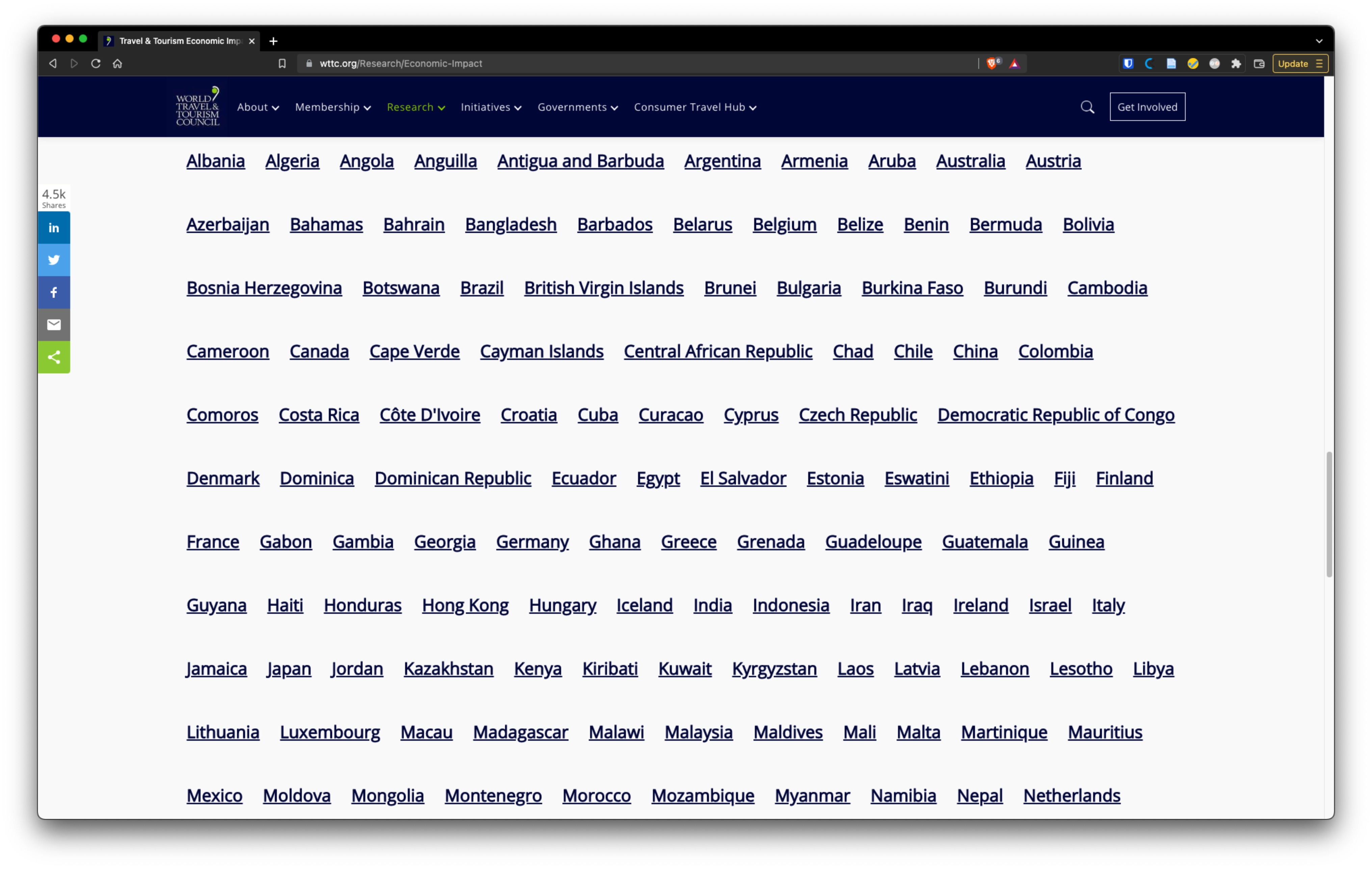
One of the component data layers of the Tourism and Recreation OHI goal is the percent of total jobs in a region that are directly tied to tourism. In the past we’ve conveniently retrieved these data from the World Travel and Tourism Council (WTTC), but this was not possible for this year’s assessment. We were able to access 2018 and 2020 tourism employment data indirectly via the World Economic Forum’s Travel and Tourism Development Index (TTDI) — however, this only provided values for countries and did not separately include the many territories we assess as part of the OHI. Fortunately, we discovered that the WTTC did provide percent change in tourism employment that we could use along with the 2019 data we already had to calculate the values we needed. The one caveat was that the percent change data were located in highly formatted tables on 185 individual PDFs, each of which are linked separately on the page shown below… This presented two options: several hours of mind numbing manual file downloading and data transcribing, or whipping up an automated scraping / extraction pipeline. The latter sounded a lot more fun.

Packages used

library(tidyverse)
library(here)
library(rvest)
library(purrr)
library(tabulizer)
library(rJava)

rvest is used to scrape the PDF download links from the webpage, purrr is used to iteratively download the files, and tabulizer is used to extract tables from the PDFs, and rJava is needed to use tabulizer.

Scraping links & downloading the files

The code below will pull all of the PDF download links from the webpage and download them to a specified directory on our machine.

We use rvest::read_html() to read the html from the webpage into an xml object in our environment. rvest::html_elements("a") is then called which finds all links within the xml object because links are denoted by the html tag <a>. To extract just the underlying URL and not the text associated with the link on the page, we use rvest::html_attr("href") — the href attribute is where the URL is specified.

We now have a vector of all the URLs linked on the page. Because there are additional links beyond just the PDFs, we need to subset the URLs. A quick look at a few of the PDF download links revealed that each has “/QuickDownload” in it. Using that pattern, we subset our vector with stringr::str_subset(), and then remove duplicated links.

The next part of the pipe sequence uses the purrr::walk2() function which iteratively passes two arguments from two lists to a particular function. Unlike purrr::map2(), walk2() returns the input .x invisibly — this is preferred as the sole outcome we want is for the files to be downloaded onto our machine. We feed in the subset of URLs, along with a vector of file names. The file names are created by extracting the unique id associated with each document from its URL and pasting it into the format {path_to_file}/wttc_{id_num}.pdf. Lastly, download.file() is passed in as the function to be applied.

When this finishes running, all the PDFs will be in the directory we created!

# pull html from the page of interest
page <- read_html("https://wttc.org/Research/Economic-Impact")

# name and create our download destination folder
pdf_dir <- here(paste0("globalprep/tr/v", version_year, "/wttc_pdfs/"))
dir.create(pdf_dir)

raw_list <- page %>% # takes the page above for which we've read the html
  html_elements("a") %>%  # find all links in the page
  html_attr("href") %>% # get the url for these links
  str_subset("/QuickDownload") %>% 
  unique() %>% 
  walk2(., paste0(pdf_dir, "wttc_", # extract unique identifier from URL for file name, and download file
                  (str_remove(., "https://wttc.org/Research/Economic-Impact/moduleId/704/itemId/") %>% 
                     str_remove("/controller/DownloadRequest/action/QuickDownload")), ".pdf"),
        download.file, mode = "wb")
        

Getting setup for our PDF scraping loop

Here we create a vector with the names of all the files we just downloaded and make an empty dataframe to be populated with the values we’ll scrape from the PDFs.

# vector of names of files we downloaded
files <- list.files(here(paste0("globalprep/tr/v", version_year, "/wttc_pdfs")))

n_countries <- length(files)

# dataframe to be populated with extracted values
tr_jobs_pct_change <- data.frame("country" = vector(mode = "character", 
                                 length = n_countries),
                                 "pct_change_2020" = vector(mode = "character", 
                                 length = n_countries),
                                 "pct_change_2021" = vector(mode = "character", 
                                 length = n_countries))

Loop to extract data from PDFs

The following loop uses tabulizer::extract_tables() to read in the data from each document as a dataframe. We then pull the values of interest from the dataframe and insert them in the final dataframe we created above.

tabulizer provides a series of R wrapper functions for the Tabula java library.

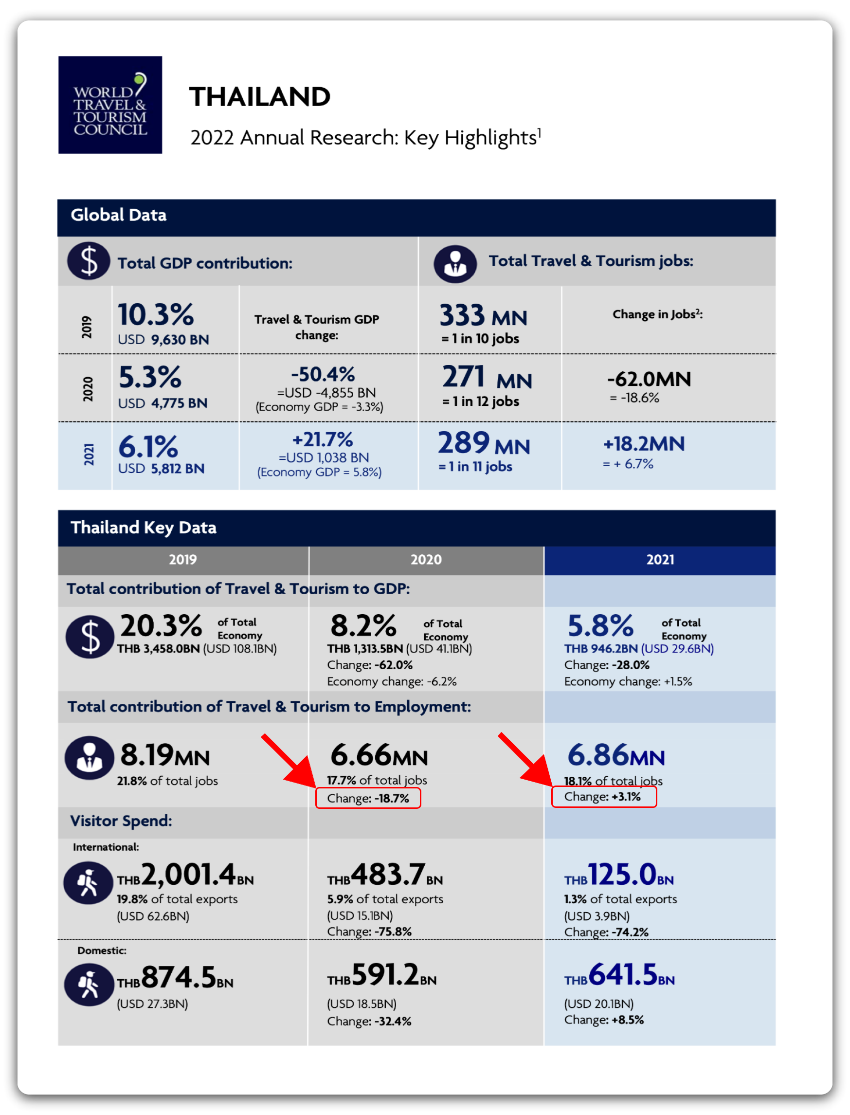
The loop passes each full file path into extract_tables(). The documents are two pages each but we only want the first, so we pass in 1 for the pages argument. The area argument can be used to specify a certain area of the document that you want to be extracted — this is done using pixel coordinates. Due to the highly formatted nature of these PDFs, doing so will help us get the best output dataframe possible, with the least amount of manipulation afterwards. There are many ways to find the pixel coordinates of a table in a PDF — I opened the file in GIMP (an open source image manipulation program similar to Photoshop) and determined the bounding coordinates there. The order of pixel bounds is top, left, bottom, right. The method argument refers to the Tabula extraction algorithm that will be used. One is optimized for spreadsheet-like documents, the other is generalized — passing in "decide" lets the function automatically determine whether the document is or isn’t spreadsheet-like.

While Tabula and the tabulizer package are incredibly powerful tools, the way these PDFs are formatted causes our output dataframes from extract_tables() to be quite disorderly. The good news is that the formatting is entirely consistent between documents, and we only need a few values from each page — so we can just index the cells that we need from the resulting dataframe despite its untidiness.

The next few parts of the loop pull out the country name and the percent change in contribution of tourism to employment, and then assign those values to a row in the final dataframe.

After this process, it was crucial to check a number of the values against what was in the PDFs to make sure everything looked correct.

for (i in seq_along(files)) {
  
  df <- extract_tables(
    file = paste0("globalprep/tr/v", version_year, "/wttc_pdfs/", files[i]), 
    pages = 1,
    area = list(c(360, 38, 1120, 770)),
    method = "decide", 
    output = "data.frame")
  
  country <- df[[1]][2, 1] %>% 
    str_remove(" Key Data")
  
  pct_change_2020 <- df[[1]][15, 1] %>% 
    str_remove("Change: ") %>% 
    str_remove("%") %>% 
    as.numeric()
  
  pct_change_2021 <- df[[1]][16, 1] %>% 
    str_remove("Change: ") %>% 
    str_remove("%") %>% 
    as.numeric()
  
  tr_jobs_pct_change[i, ] <- c(country, pct_change_2020, pct_change_2021)
  
}

Export dataframe as a CSV and delete PDFs

Now we can just save our dataframe as a CSV and get rid of all the PDFs.

write_csv(tr_jobs_pct_change, here(paste0("globalprep/tr/v", version_year, "/intermediate/tr_jobs_pct_change.csv")))

# delete all downloaded pdfs
unlink(pdf_dir, recursive = TRUE)

Conclusion

In theory, if the WTTC uses this same format for their reports in future years, this workflow could be reused as is. If not, we would likely only need to change the pixel coordinates and the row/column indices used to get the desired values. Either way this was a fun project that saved us from monotonous work and may continue do so for future fellows!